INCAM 2026 · Submitted

PyAMorph: High-Fidelity Implicit Geometry
Modeling and Morphometric Analysis
on Adaptive Meshes

A massively parallel Python framework combining Signed Distance Functions, Constructive Solid Geometry, and AMReX Adaptive Mesh Refinement for simulation-ready microstructure analysis.

Harshdip Sahaa  ·  Anshika Singha  ·  Zeeshan Ahmada  ·  Ark Malhotraa  ·  Rashmi Chaudhrya  ·  Pradeep Kumar Seshadrib,*

a Netaji Subhas University of Technology, Delhi b Indian Institute of Technology, Madras
Read Abstract Explore Gallery

Abstract

The macroscopic performance of heterogeneous systems — such as the regression rates of solid propellants or the stiffness of architected metamaterials — is intrinsically linked to the topology of microstructures. In these domains, geometric fidelity directly determines the accuracy of predicted physics, including flame-front evolution and localised stress concentrations. Current computational pipelines either impose prohibitive memory costs via uniform fine grids, or sacrifice resolution through aggressive coarsening.

To bypass this resolution-memory trade-off, we introduce PyAMorph, a massively parallel adaptive framework for multi-source implicit modelling and morphometry. Utilising Signed Distance Functions (SDFs) within a unified Constructive Solid Geometry (CSG) environment, the framework integrates disparate data sources — including noisy volumetric images, STL manifolds, and analytical functions. By building on hierarchical AMReX MultiFab structures with Adaptive Mesh Refinement, the zero-level set is resolved at high fidelity while bulk phases remain coarser, enabling scalable domain decomposition without memory bottlenecks.

01

Package Overview

pySdf is organised into four modular packages, each with a consistent operator-based API. All geometry classes support | (union), - (subtraction), and / (intersection) operators, and produce NumPy arrays or AMReX MultiFabs.

~50 shapes

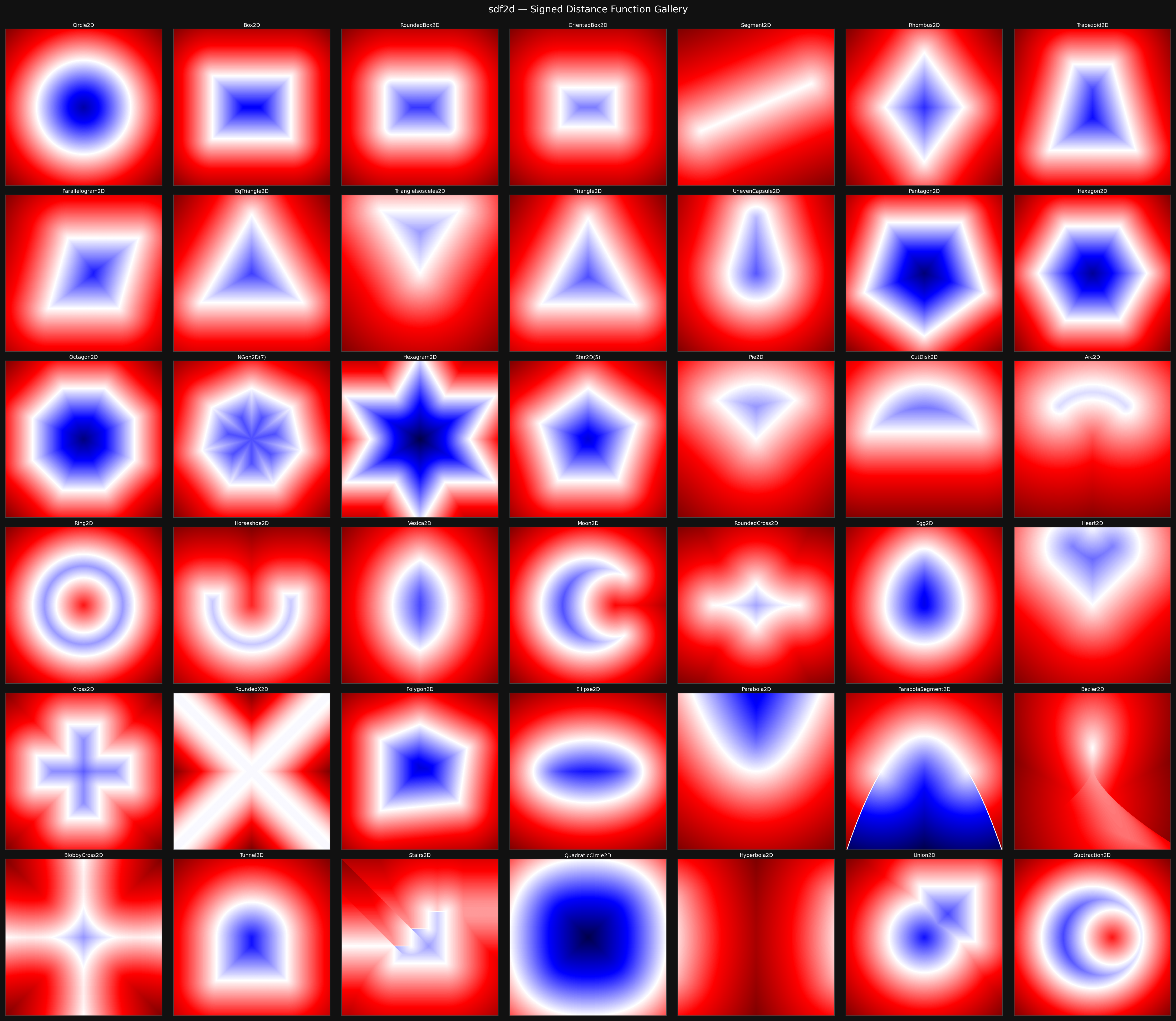
sdf2d

2D geometry classes, grid sampling, and optional AMReX MultiFab output. Includes Circle2D, Box2D, Hexagon2D, and dozens more.

~30 shapes

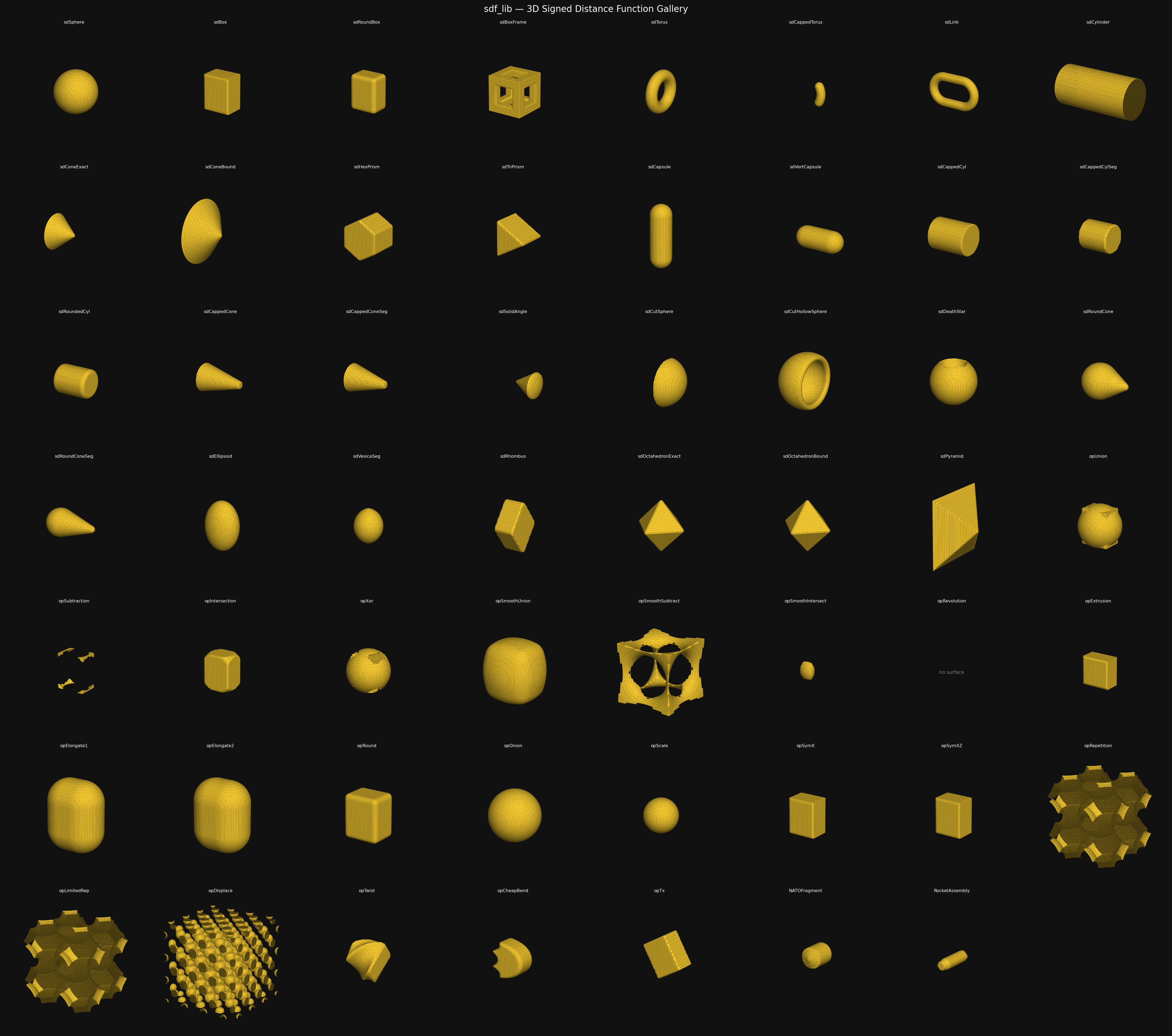
sdf3d

3D geometry classes, TPMS metamaterials, spatial warp operators, and AMReX output. Includes Sphere3D, Box3D, Torus3D, and lattice structures.

STL → SDF

stl2sdf

Convert any watertight STL mesh into a composable SDF3D using the Ericson closest-point algorithm and Möller–Trumbore sign detection. Pure NumPy.

Image → SDF

img2sdf

2D image or 3D volume → SDF via True 3D Robust Chan-Vese segmentation. Computes morphometric descriptors: volume, surface area, sphericity, curvature, and more.

Sign convention:  φ < 0 inside the solid,  φ = 0 on the surface,  φ > 0 outside. Primitive analytic shapes are true SDFs (|∇φ| = 1). After boolean operations or image-derived fields the result is a levelset.
03

TPMS Metamaterials

Triply Periodic Minimal Surfaces and beam lattices are first-class SDF3D subclasses. They accept cell_size, thickness, and repeat=(rx, ry, rz) for tiling, and compose with all analytic primitives via the same | / - / / operators.

Gyroid3D

Gyroid

sin x·cos y + sin y·cos z + sin z·cos x = 0

SchwarzP3D

Schwarz P

cos x + cos y + cos z = 0

SchwarzD3D

Schwarz Diamond

sin x·sin y·sin z + sin x·cos y·cos z + … = 0

Neovius3D

Neovius

3(cos x + cos y + cos z) + 4 cos x·cos y·cos z = 0

BCCLattice3D

BCC Beam Lattice

Body-centred cubic strut network

FCCLattice3D

FCC Beam Lattice

Face-centred cubic strut network

Python — Morphometric Analysis on a Gyroid
from sdf3d import Gyroid3D
from img2sdf import compute_morphometry_3d

# One unit cell, 0.3 shell half-width
gyroid = Gyroid3D(cell_size=2.0, thickness=0.3, repeat=(1, 1, 1))

metrics = compute_morphometry_3d(
    gyroid,
    bounds=((-1, 1), (-1, 1), (-1, 1)),
    resolution=(64, 64, 64),
)
print(f"Volume:       {metrics['volume']:.4f}")
print(f"Surface area: {metrics['surface_area']:.4f}")
print(f"Sphericity:   {metrics['sphericity']:.4f}")

TPMS Isosurface Gallery

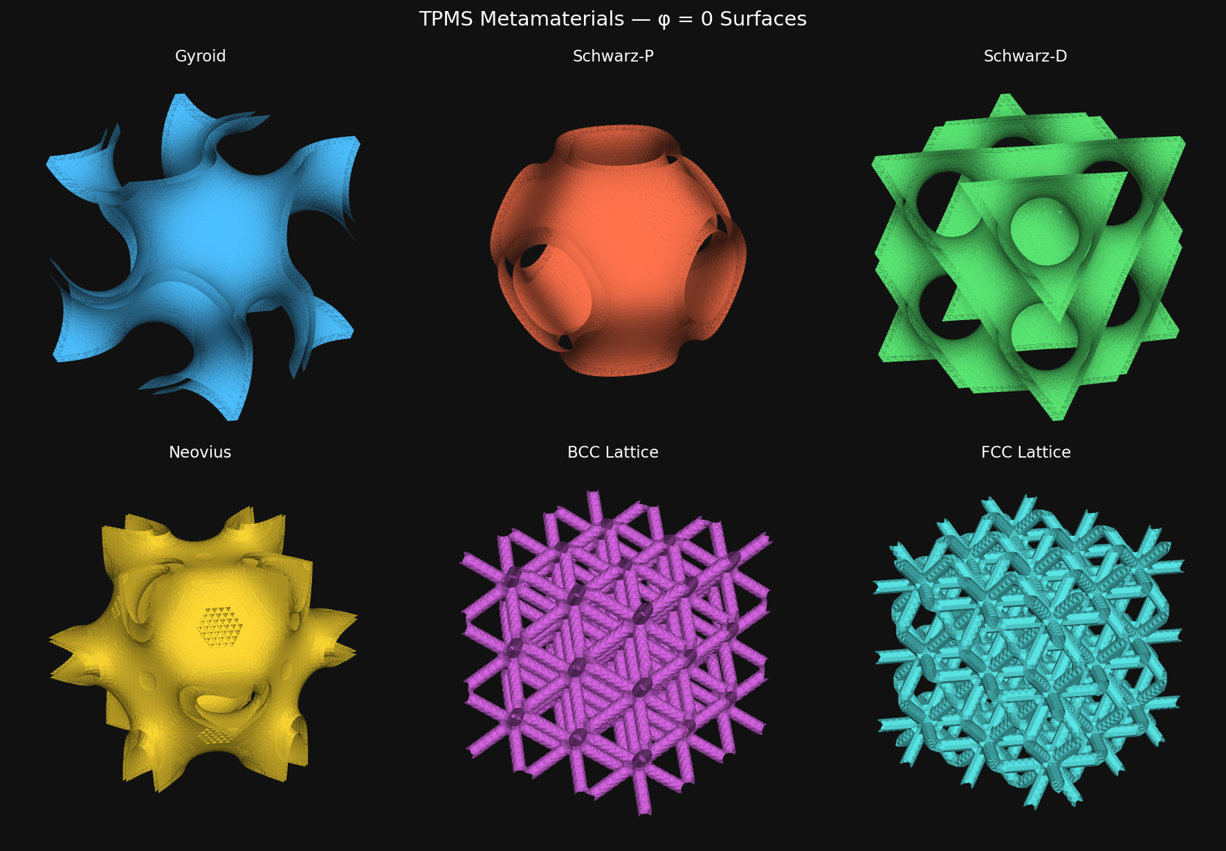
TPMS metamaterial gallery: Gyroid, Schwarz-P, Schwarz-D, Neovius, BCC Lattice, FCC Lattice
FIG 3.1 φ = 0 isosurfaces for all six metamaterial classes at unit-cell scale. Gyroid, Schwarz-P, Schwarz-D, and Neovius are triply periodic minimal surfaces; BCC and FCC are beam-network lattices. Every class is a first-class SDF3D subclass composable with any analytic primitive or image-derived field.
04

Methodology

The PyAMorph pipeline transforms raw volumetric data into simulation-ready implicit domains through a multi-stage variational approach, culminating in scalable AMReX output.

STEP 01

Segmentation

True 3D Robust Chan-Vese active contour evolves a level-set to minimise an energy functional, suppressing image noise to produce a precise SDF (φ < 0 inside solid).

STEP 02

CSG Composition

Image-derived SDFs are freely composed with analytic primitives and STL meshes using union, subtraction, and intersection in a unified CSG scene graph.

STEP 03

AMR Evaluation

Composite fields are evaluated onto hierarchical AMReX MultiFab structures. AMR resolves the zero-level set at high resolution; bulk phases remain coarser.

STEP 04

Morphometry

Morphometric descriptors — volume, surface area, sphericity, curvature, mean aspect ratio, nearest-neighbour distances, and Voronoi cell volumes — are extracted automatically.

Chan-Vese Segmentation Output (Microstructure)

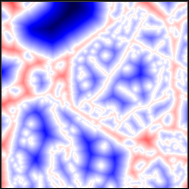
2D SDF derived from HEDS porous micrograph via Chan-Vese segmentation
FIG 4.1 SDF field recovered from a cross-sectional HEDS porous-solid micrograph via True 3D Robust Chan-Vese segmentation. Blue = solid phase (φ < 0), red = void (φ > 0), white contour = zero-level set.

STL to SDF

Python
from stl2sdf import stl_to_geometry

# Convert any watertight STL mesh → composable SDF3D
geom = stl_to_geometry("my_mesh.stl")

# Compose with analytic shapes
from sdf3d import Sphere3D
result = geom - Sphere3D(0.2).translate(0, 0, 0.3)
phi    = result.to_numpy(bounds=((-1,1),(-1,1),(-1,1)), resolution=(64,64,64))
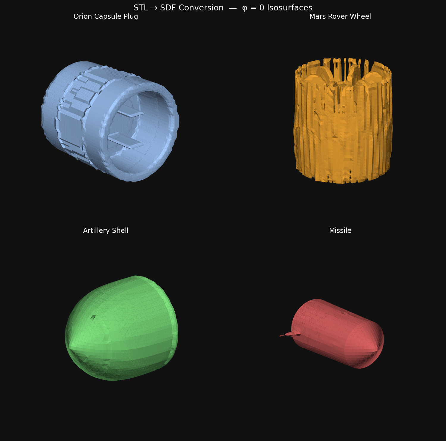
Four STL meshes converted to SDF isosurfaces: Orion capsule plug, Mars rover wheel, artillery shell, missile
FIG 4.2 Four STL meshes converted to SDF3D via stl_to_geometry() using the pysdf C++ BVH back-end. Top-left: NASA Orion capsule plug (~2 K triangles). Top-right: NASA Mars Curiosity rover wheel (~45 K triangles). Bottom: artillery shell and missile geometries. Each resulting SDF3D is fully composable with analytic primitives and TPMS metamaterials.

AMReX Adaptive Mesh Output

Python
import amrex.space3d as amr
from sdf3d import Sphere3D, Box3D, MultiFabGrid3D

amr.initialize([])
try:
    real_box = amr.RealBox([-1,-1,-1], [1,1,1])
    domain   = amr.Box(amr.IntVect(0,0,0), amr.IntVect(63,63,63))
    geom     = amr.Geometry(domain, real_box, 0, [0,0,0])
    ba       = amr.BoxArray(domain); ba.max_size(32)
    dm       = amr.DistributionMapping(ba)

    grid  = MultiFabGrid3D(geom, ba, dm)
    mf_a  = Sphere3D(0.3).to_multifab(grid)
    mf_b  = Box3D((0.2, 0.2, 0.2)).to_multifab(grid)
    mf_u  = grid.union(mf_a, mf_b)       # min(a, b)
    mf_s  = grid.subtract(mf_b, mf_a)    # box with sphere carved out
finally:
    amr.finalize()
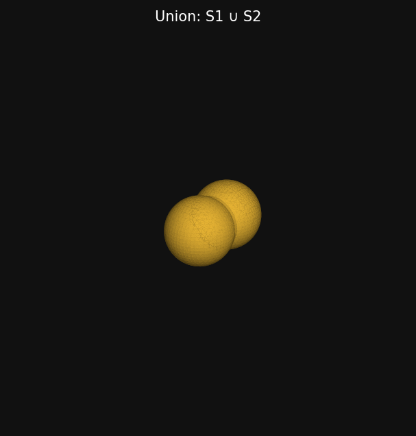
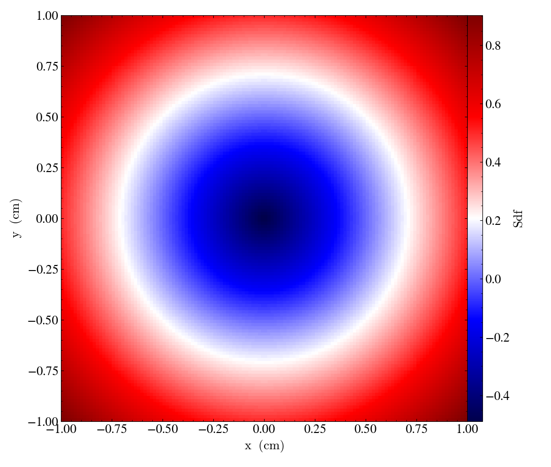
AMReX MultiFab SDF field — circle union, blue inside red outside
FIG 4.3 AMReX MultiFab output: SDF field of a Circle2D evaluated onto a uniform grid. Blue = inside (φ < 0), red = outside (φ > 0).
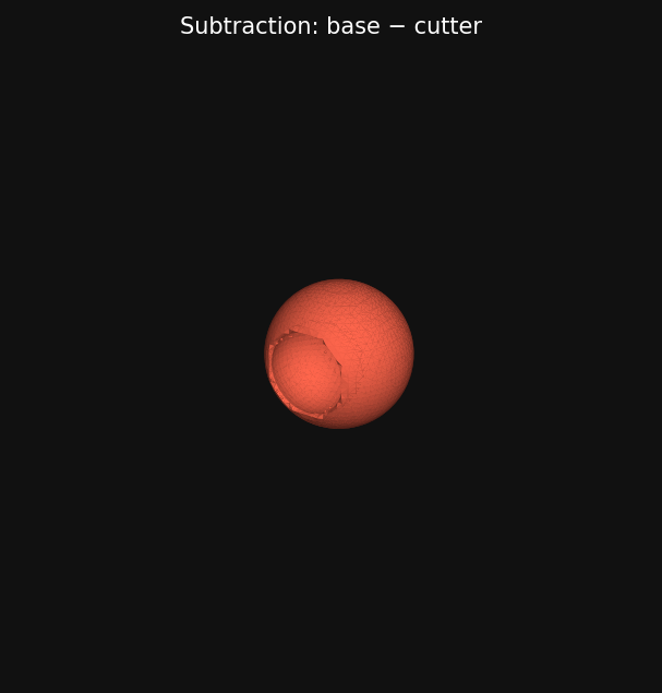
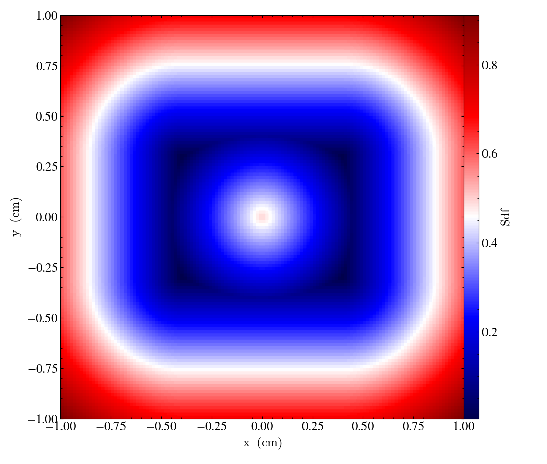
AMReX MultiFab SDF field — rounded box with spherical cavity
FIG 4.4 AMReX MultiFab output: SDF of a rounded box with a spherical cavity subtracted at its centre, demonstrating CSG subtraction on an AMReX grid.
05

Results

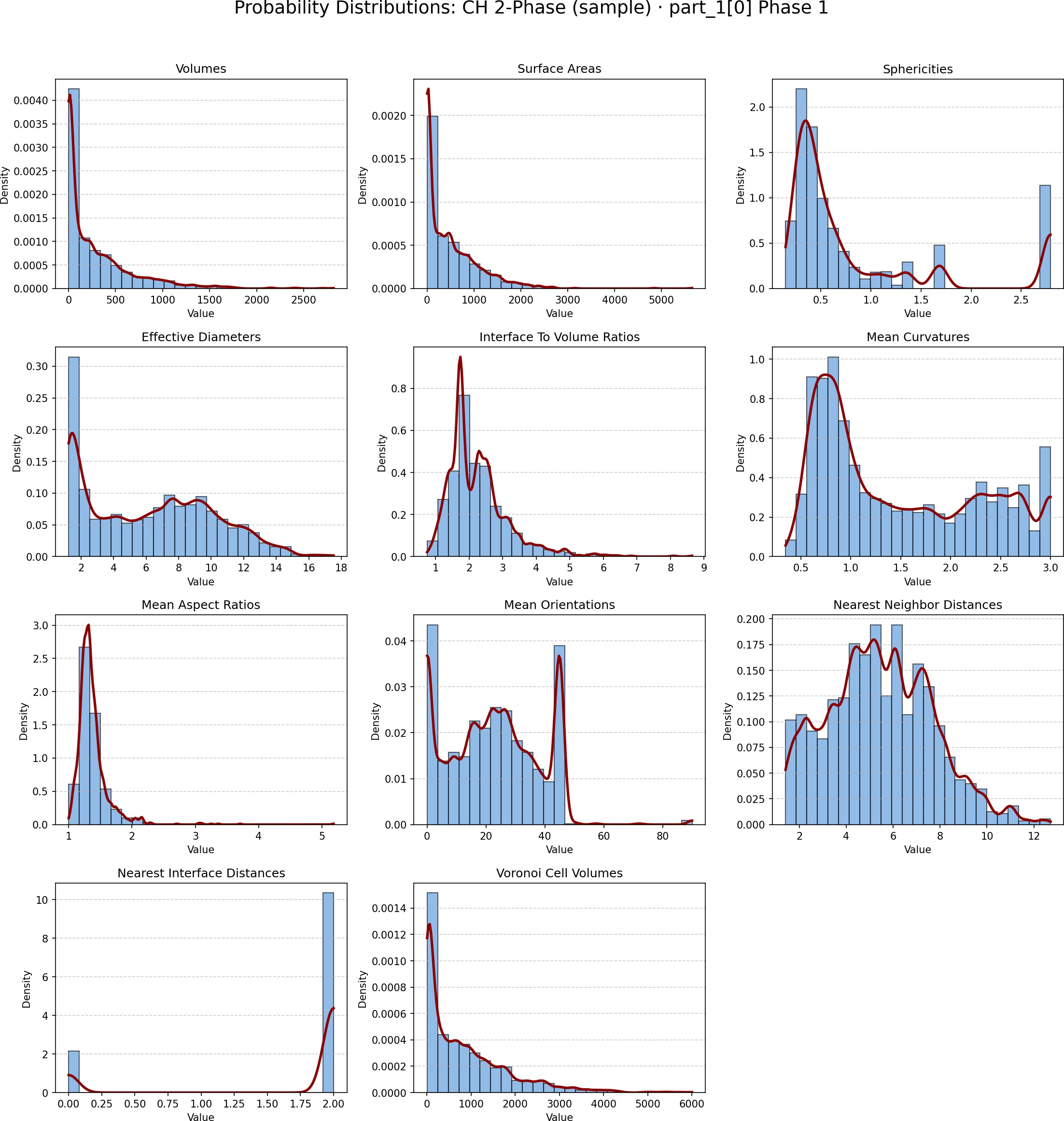
PyAMorph successfully demonstrated high-fidelity reconstruction and automated statistical characterisation of complex porous microstructures. The framework extracted 11 morphometric distributions per phase over an ensemble of segmented volumes.
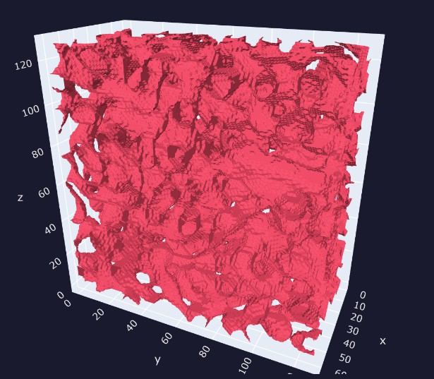
3D porous microstructure reconstructed via Chan-Vese segmentation
FIG 5.1 3D porous microstructure generated via True 3D Robust Chan-Vese segmentation (φ < 0 inside). Rendered as a marching-cubes isosurface on an AMReX MultiFab grid.
Probability distributions of morphometric descriptors
FIG 5.2 Probability distributions of 11 morphometric descriptors (CH 2-Phase segmentation). KDE curves (red) are fitted to each descriptor across the particle ensemble.
V

Volume

Voxel-summed solid phase volume per particle

A

Surface Area

Marching-cubes triangle area integration

ψ

Sphericity

Ratio of sphere surface area to actual surface area

d

Eff. Diameter

Equivalent sphere diameter from volume

κ

Mean Curvature

Integrated mean curvature over the surface

α

Aspect Ratio

Bounding-box principal axis ratio
3D porous solid-phase isosurface — full volume reconstruction
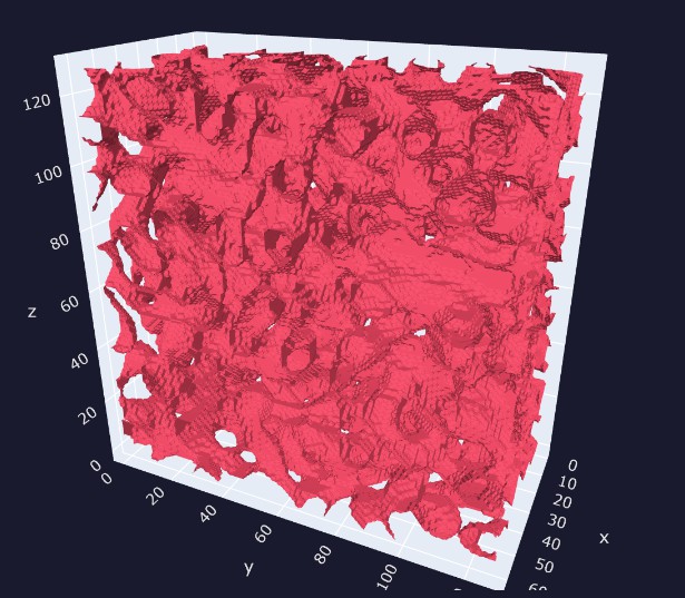
FIG 5.3 Solid-phase isosurface of the full 3D reconstructed volume (CH 2-Phase). The irregular pore network topology is faithfully captured by the zero-level set.
Probability distributions of 11 morphometric descriptors — Phase 1
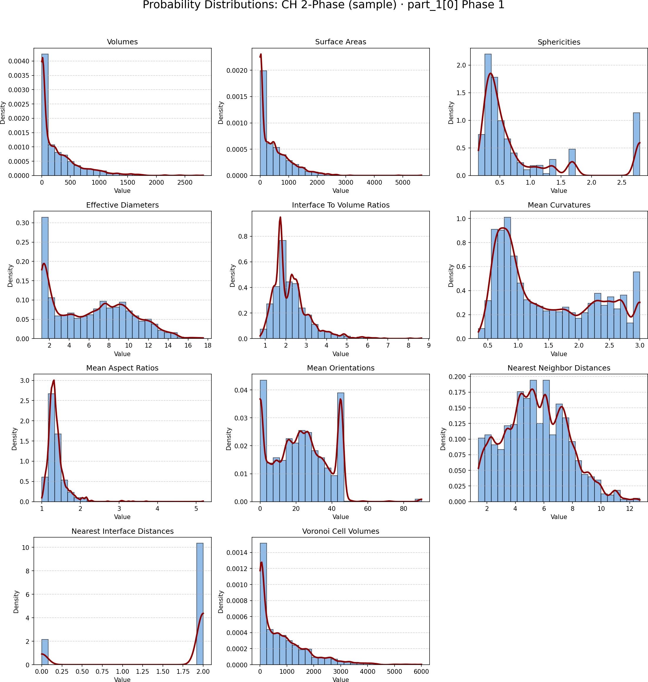
FIG 5.4 Probability distributions of 11 morphometric descriptors for Phase 1 particles. KDE curves (red) are fitted to each descriptor across the full particle ensemble.